As I’ve hinted in the past (e.g., here and here), I really love a good map. Lately, a few colleagues have approached me for help with mapmaking. Despite each person’s focus on a different region or topic, I’ve found that the same small set of free online resources have usually proved to be equal to the task.
Generally, my approach is to collect high quality vector data for map features such as political boundaries, rivers, or roads. These are often available for the GIS community in shapefile format or some other widely supported vector format. I then plot the data in R using the maptools package. R is more than capable of putting together beautiful maps and is far more lightweight and efficient than dedicated GIS programs. It also runs on every operating system. For Mac/Linux users, no need to fiddle with virtual machines, dual boot machines, or other people’s machines just for access to ArcGIS!
Here are some websites to bookmark:
Natural Earth
Natural Earth is usually my first stop for free general-purpose spatial data for cartography. It offers global cultural and physical vector data at three different scales, as well as raster data at two scales. For certain datasets, multiple options are presented, giving more control over the features actually downloaded. Best of all, the features are quite up-to-date. One of my major complaints about mapping in R was the datedness of the data included in widely used packages such as maps and maptools, both of which use the CIA World DataBank II, which was last updated in the 1980s!
DIVA-GIS
DIVA-GIS provides a portal to free spatial data hosted around the web. I find the country-level data particularly useful and use it often, particularly when my focus is on one or a few countries.
Protected Planet
Protected Planet provides very good vector data for protected areas of the world. The global dataset is available for download but is enormous at nearly 3 gigabytes. It is usually more useful to download data by country.
Global Land Cover Facility
I focus on vector data for my cartographic needs, but on the rare occasions when I need raster data I turn first to the Global Land Cover Facility (GLCF) at the University of Maryland, which provides useful raster data including satellite imagery and earth science products derived from satellite imagery.
Socioeconomic Data and Applications Center
In a similar vein, the Socioeconomic Data and Applications Center (SEDAC) at Columbia University provides useful census (population) data in raster form.
ColorBrewer
Unlike the other resources on this list, ColorBrewer does not provide any data. It does, however, offer excellent guidance for color usage in maps. The user can specify her data nature, pick a color scheme, and generate a set of colors tailored to her purpose. She can even filter only colorblind safe, printer friendly, or photocopy safe color schemes. Colors are provided as Hex, RGB, or CMYK values.
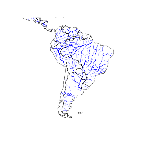
To demonstrate how easily and quickly maps can be put together, I decided to create a map of South American rivers. To do this, I downloaded global national borders (110m resolution) and global rivers (110m, 50m, and 10m resolution) from Natural Earth. I then plotted all the features in R.
library('maptools')

# Set the WGS84 projection for all features
options(proj4string=CRS('+proj=longlat +datum=WGS84'))

world <- readShapePoly('ne_110m_admin_0_countries.shp')
water1 <- readShapeLines('ne_110m_rivers_lake_centerlines.shp')
water2 <- readShapeLines('ne_50m_rivers_lake_centerlines.shp')
water3 <- readShapeLines('ne_10m_rivers_lake_centerlines.shp')

# Plot water features with three different line weights
plot(water1,add=FALSE,col='blue',lwd=2,xlim=c(-75,-50),ylim=c(-55,15))
plot(water2,add=TRUE,col='blue',lwd=1)
plot(water3,add=TRUE,col='blue',lwd=0.25)
plot(world,add=TRUE,lwd=1)
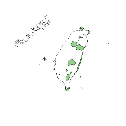
Next, I decided to create a map of Taiwanese national parks using global national borders (10m resolution) from Natural Earth and protected areas of Taiwan from Protected Planet.
world.hires <- readShapePoly('ne_10m_admin_0_countries.shp')
taiwan.parks <- readShapePoly('general_TWN-shapefile-polygons.shp')

plot(world.hires,xlim=c(118.5,123),ylim=c(21.25,25.75))
plot(taiwan.parks,add=TRUE,col='#a1d99b')

 RSS
RSS